helps to separate ice from snow because both ice and snow
have unique spectral signatures in the
VIN
region (Ambi-
nakudige and Joshi, 2012; Racoviteanu
et al.
, 2008). We used
a threshold value of 202 on the values of above band ratio
(values ranged from 0 to 255) to separate ice and snow. Last,
we classified water and debris manually and excluded those
classes from the analysis. After the final image classification,
in ArcGIS
®
10.2 software, we overlaid the
ICESaT
footprints
on the classified image and extracted classified pixel values.
We used a total of 138,763 elevation footprints in the analy-
sis. Of these footprints, 113,951 elevations were outside the
glaciers, 12,009 were on clean ice, 11,279 were on glacier firn/
snow, and 1,524 were on debris-covered ice. There were 2,119
footprints in
DC
, 5,538 in
NW
, 5,741 in
SPI
, and 1,421 in
CDI
regions.
After the extraction of land cover classes from overlaying
pixel to the
ICESaT
footprints, we also extracted the elevation
values from the
SRTM DEM
using the bilinear interpolation
technique. Then we calculated elevation differences per year
by subtracting
ICESaT
(from the years 2004 to 2008) elevation
and
SRTM
elevation (from 2000) in the clean ice zone during
the dry season. We removed points with elevation differences
greater than +150 and less than −150, because we assume that
these are possible errors in the data due to clouds or other fac-
tors (Kääb
et al.
, 2012; Phan
et al.
, 2014). Finally, we used the
remaining footprints to calculate the trends in the elevation
differences over the study period.
We computed uncertainty in the trend estimation (
u
) as the
root sum square of the standard error of elevation difference
trends in glacier (
SE
gl
), elevation difference trends outside gla-
ciers (
EDT
nongl
) as shown in Equation 1 (Gardner
et al.
, 2013;
Kääb
et al.
, 2012; Neckel
et al.
, 2014):
u SE EDT
gl
nongl
=
+
2
2
(1)
To prepare the parameters for Equation 1, we conducted a
bootstrap analysis to examine the possible error introduced
in the analysis due to the uneven number of sample points
in each year. From the elevation difference footprints on
glaciers, we randomly selected points for bootstrap analysis
with an increment of 10 percent points at each stage, until we
covered 100 percent points. We used two hundred iterations
at each stage (Kääb
et al.
, 2012; Neckel
et al.
, 2014). We fitted
a second-order polynomial through all the standard devia-
tions of the elevation difference trend values obtained from
the bootstrap analysis. We then used the fitted polynomial
value at the 100 percent points in calculating standard error
(
SE
gl
) and used in equation 1(Kääb
et al.
, 2012; Neckel
et al.
,
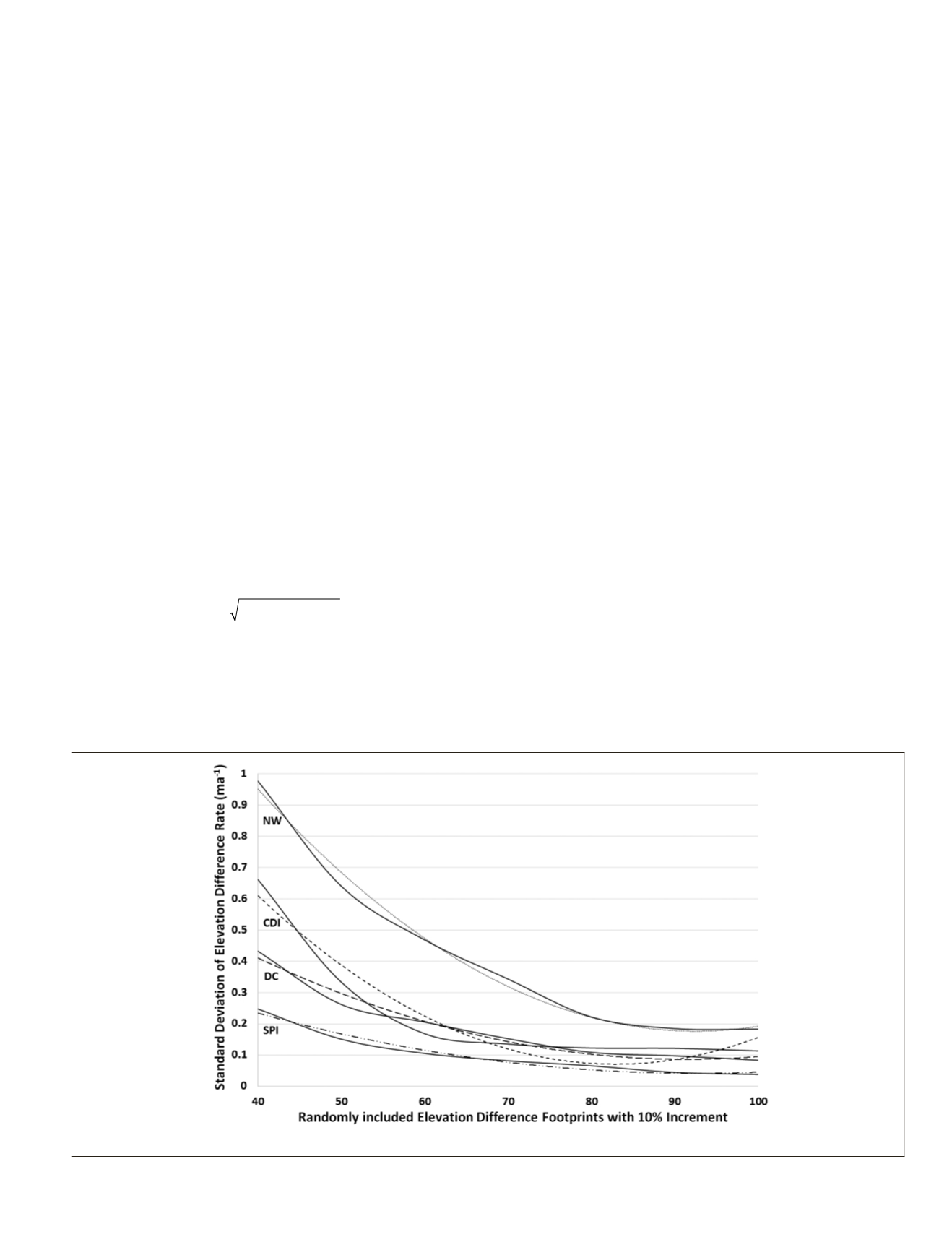
2014). We noticed representativeness of elevation footprints
varies in the regions. In all regions except the
NW
, standard
deviation values leveled off at around 55 percent of the points
(Figure 4). In the
NW
region, standard deviation values leveled
off at around 80 percent points (Figure 4). We therefore used
the standard deviation value at 100 percent footprints in the
uncertainty estimation.
The accuracy of the
ICESaT
’s altimetry elevation measure-
ment in the high slope areas is very low (Carabajal and Hard-
ing, 2006; Kääb
et al.
, 2012; Neckel
et al.
, 2014). Therefore, to
get the precise error estimates in elevation differences in off-
glacier areas, we fitted a linear trend on elevation differences
in off-glacier footprints in areas where slope values are less
than 10 degrees. We then used this trend value (
EDT
nongl
) in
Equation 1. Although studies have noted that there could be
inter-annual biases of about ±0.03 to 0.06 m a
-1
in the
ICESaT
laser period (Gardner
et al.
, 2013), we assume that our un-
certainity estimation method is inclusive of any inter-annual
biases. Finally, we computed glacier mass balance trend and
associated uncertainty by multiplying a density value of 900
kg m
−3
for clean ice (Huss, 2013).
Results and Discussion
The trends of elevation differences indicate varied glacial
wastage rates throughout the study period. Figure 5 depicts
the glacial thinning trends in
DC
,
NW
,
SPI
, and
CDI
regions on
clean ice areas. We calculated these trends by fitting a linear
model through all available elevation differences in
ICESaT
footprints from 2004 to 2008 with respect to year 2000
SRTM
elevation values. We fitted these trends through all footprints
that fall within one and two standard deviations from the
mean. We calculated the elevation difference trends and mass
balance trends using all points. Figure 5 shows the trends of
elevation differences fitted through all points.
Figure 4. Trends of standard deviation of elevation differences from randomly selected points over clean ice.
PHOTOGRAMMETRIC ENGINEERING & REMOTE SENSING
October 2016
815


