In the first stage, the lidar point cloud is tessellated into
0.5 m × 0.5 m cells across the horizontal plane. Each cell is
identified by a unique (row, column) index. Based on the
cluster of points within each cell, the point with the lowest
height is initially labeled as ground and is denoted by
P(i,j)
.
Due to underbrush, not every point selected in the previ-
ous step represents true ground. Therefore, the second stage
involves coding a variety of features to represent attributes
of each lowest point
P(i,j)
and the lowest points in each of
the neighboring columns. Table 1 lists the eight features used
to discriminate ground from non-ground. These features
are combined into a feature vector
F(i,j)
for each point that
is used by the
SVM
classifier to identify whether that point
belongs to ground or not.
The
SVM
classifier is trained given the feature vectors in Ta-
ble 1 and the hand-attributed labels of each point
P(i,j)
that lies
on the ground surface. If a cell contains a point labeled by the
classifier, it is treated as true ground. Delaunay triangulation is
performed for cells that do not have points not yet labeled.
The next step involves identifying the vertical extents of
stems using thresholding and clustering methods. To iden-
tify which lidar point belongs to the main stem, a simple
height-above-ground filter is used. Any point below the select-
ed height threshold is discarded and classified as underbrush.
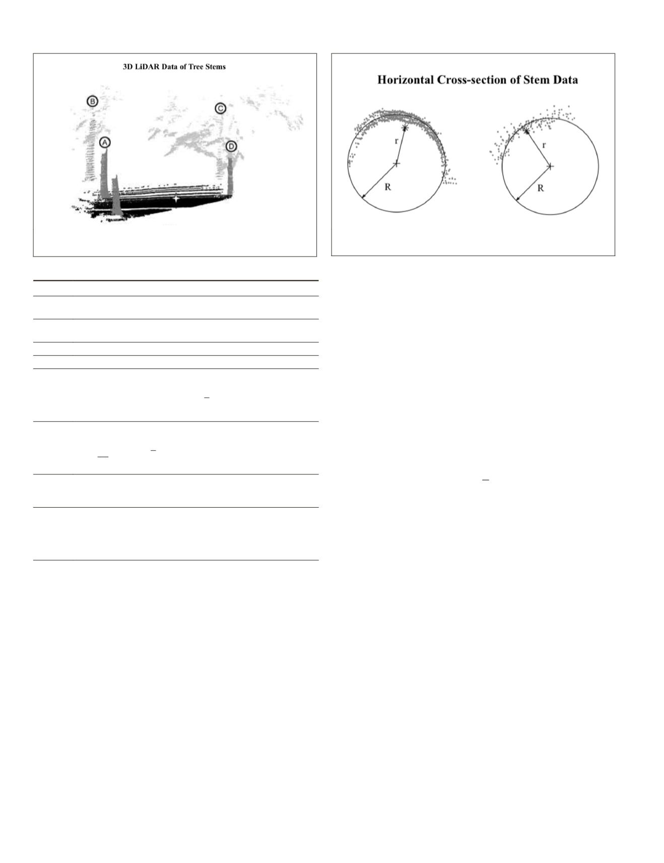
Figure 3 shows a group of tree stems and the ground plane
as modeled by lidar. Based on the dataset obtained and the
vertical extents of observed underbrush, we empirically deter-
mined that a height threshold of 2 m is adequate. Filtered data
is then clustered following a single-linkage clustering method,
which classifies two points to belong to a single cluster if they
are within a predefined distance.
Finally, cylinder primitives are fitted to filtered lidar data
using a least squares scheme. Figure 4 shows how a cylinder
primitive is fit to a horizontal slice of 3
D
lidar data pertaining
to a tree stem.
R
denotes the radius of the base of the cylinder
primitive while
r
denotes the estimated radius of curvature of
the stem slice containing lidar data. The fit between the cyl-
inder primitive and data is found by minimizing the squared
distance error below.
arg
min
d
x
i
n
i
∈
=
=
( )
∑
R
3
1
2
1
2
x
(1)
where
n
is the number of points in a cluster,
x
is the transect
containing lidar points pertaining to the identified stem, and
d
i
is the Euclidean distance from the
i
th
point to the surface of
the cylinder primitive.
Following the minimization step, horizontal locations
of tree stem centers relative to the rover are determined by
calculating the radius of curvature of each fitted cylinder. The
location of each estimated tree center in the horizontal plane
is incorporated into a tree center map for each pose.
Matching of Tree Centers from Overhead
Imagery and Rover Lidar Data
The third component of the algorithm has the primary func-
tion of matching local tree center maps obtained from ground
lidar to a constellation map of stems to estimate the hori-
zontal geoposition of the rover. Most of registration prob-
lems employ some variant of the Iterative Closest Point (
ICP
)
algorithm. Examples include Trimmed
ICP
(Chetverikov
et al
.,
2002), Multi-scale
ICP
(Granger and Pennec, 2002) and Gauss-
ian
ICP
(Jian and Vemuri, 2011). Such methods are capable of
discarding outliers and producing a best fit based on a statisti-
cal filtering approach to noisy data. In fact, tree center maps
generated from overhead image data include outliers due to
the presence of complex crown profiles that results in over
segmentation of the imagery. Robust registration therefore
becomes important in our case to avoid inadvertent errors in
geoposition estimates.
T
able
1. SVM C
lassifier
F
eatures
Feature Description
F
1
Number of occupied columns in the neighborhood of
column
(i,j)
F
2
Minimum height of all neighbors minus height of column
at
(i,j)
F
3
Value of height at column
(i,j)
F
4
Average of all heights in neighborhood of column
(i,j)
F
5
Normal to best fit plane of points in neighborhood to
column
(i,j)
. Defined as:
F
n n
k
N
5
1
1
2
3 2
=
−
(
)
(
)
∈ =
=
∑
argmin
,
R
P P n
k
.
F
6
Residual sum of squares of best fit plane of points in
neighborhood of column
(i,j)
F
N
k
N
6
1
2
1
=
−
(
)
(
)
=
∑
P P n
k
.
F
7
Pyramid filter is used where feature is computed as the
number of minimum heights which lie within a pyramid
of 0.5 m cubic voxels with apex at
P(i,j)
F
8
Ray tracing score where points lying on flat ground are
given a zero score because they cannot lie between the
lidar and any point it sees. This feature is defined as the
sum of the number of line segments that pass through a
voxel in column
(i,j)
below
P(i,j).
Figure 3. 3D Lidar Data Showing Profile of Tree Stems and the
Ground Plane (McDaniel, 2010).
Figure 4. Example Showing Cylinder Fitment to a Single Slice of
3D Lidar Data of Tree Stems (McDaniel, 2010).
842
November 2015
PHOTOGRAMMETRIC ENGINEERING & REMOTE SENSING


