point is found in the search window in the right image by the
FBM
, then the
ABM
implemented by the
NCC
is adopted. The
threshold of the correlation coefficient is also set to 0.8.
After
FBM
and
ABM
, the two sets of the corresponding fea-
tures obtained from the bi-directions of the left and right im-
ages are merged. Special consideration is given to redundant
point elimination and efficiency. The use of the two different
matching techniques may potentially provide different levels
of precision in the image and object spaces. The
FBM
method,
which is based on the
SIFT
operator, yields a precision of
0.3 to 0.5 pixels in the image space (Barazzetti
et al
., 2010).
However, the
NCC
technique can attain a precision of 0.1 to
0.3 pixels when the standard algorithm is integrated with the
interpolated correlations in the neighborhood of the maxi-
mum value using a polynomial function (Grün, 2012). In both
cases, subpixel precision can be achieved, which is sufficient
for the application being considered. The matched-feature
point pairs are then used to calculate the 3D object positions
by applying the photogrammetric forward intersection algo-
rithm (Cooper and Robson, 1996). The residual of the spatial
intersection of the two rays projecting from the corresponding
image points to the ground point in the object space is used as
an uncertainty indicator and verified against a threshold for
accepting or rejecting the matched-image feature pair.
Velocity Estimation from Tracked Features
If a sliding feature extracted from the stereo-image pair (Image
I
k
, Image
J
k
) is successfully matched, then its 3D position can
be determined as
P
k
with coordinates (
X
k
, Y
k
, Z
k
). Similarly, if
the same sliding feature is tracked at subsequent time
k+1
and
matching is successfully performed in the stereo pair (Image
I
k+1
, Image
J
k+1
), then its position can be determined as
P
k+1
with coordinates (
X
k+1
, Y
k+1
, Z
k+1
). The direction of the veloc-
ity is then estimated on the basis of the 3D coordinates
P
k
and
P
k+1
. The speed can be calculated as:
speed
X X Y Y Z Z
f
k
k
k
k
k
k
=
− + − + −
+
+
+
(
) (
) (
)
/
1
2
1
2
1
2
1
(2)
where
f
is the image acquisition rate.
Experimental Results and Discussion
Experiment Setup
In this study, we report the results from a landslide simula-
tion experiment designed to investigate the proposed dynamic
photogrammetric image-processing methodology for landslide
monitoring. For a more detailed description of the simulation
facility and other contact sensor experiments and their physi-
cal interpretations, refer to Scaioni
et al
. (2013) and Lu
et al
.
(2015). This landslide simulation experiment lasted for approx-
imately four hours and 50 minutes. At the beginning of the ex-
periment, the accelerated rainfall rate was set to 60 mm/h and
was then gradually increased to 150 mm/h to simulate heavy
rainfall, which would rapidly trigger a landslide in the simula-
tion environment. The accumulated rainfall was approximately
240 mm according to the record of the rain gauge. This type of
the heavy precipitation can be reached during the rainy season
based on recent meteorological records in mountain areas of
western China. For example, an accumulative rainfall of ap-
proximately 330 mm in 40 hours during a rainstorm event from
23 to 24 September in 2008 induced 969 new landslides in a
Beichuan study area in the region of the Wenchuan Earthquake
(Tang
et al
., 2011). Compared to this actual landslide triggering
event, the ratio of the simulation periods is about 1:8.3 and that
of the accumulative rainfall 1:1.4. If we define a compound en-
largement factor by a product of the simulation period and the
accumulative rainfall, its calculated value is about 1:12. The
area of the simulation slope is 9 m
2
and the targeted field land-
slide body should have a dimension of around 108 m
2
(9 m
2
×
12), which fits the most frequent landslide dimension category
of 100 m
2
to 500 m
2
in the Taziping region (Qiao
et al
., 2013).
During this process, the contact sensors were activated to col-
lect different geotechnical parameters and geometrical deforma-
tion measurements. When the landslide mass was soaked, the
landslide body began to move increasingly rapidly until slope
failure. The
SLRC
camera was used to collect the single-image
sequence at a frequency of six frames per minute for the last
two and half hours because of a technical problem. When the
rainfall rate was increased and the slope became unstable, the
HSCS
cameras began recording the stereo-image sequence at a
frequency of 20 frames/S. A total of 738 sequential images from
the
SLRC
images and 95 sequential stereo-image pairs from the
HSCS
were captured. The two
HSCS
cameras were synchronized
by the hardware. The specifications of the camera systems and
experimental settings are listed in Table 1.
Event Detection During the Entire Landslide Process Based on Single
SLRC Image Sequences
Both the altered features and sliding blocks derived from the
single
SLRC
image sequence through FPT were used to detect
pre-failure events and the main slope collapse throughout
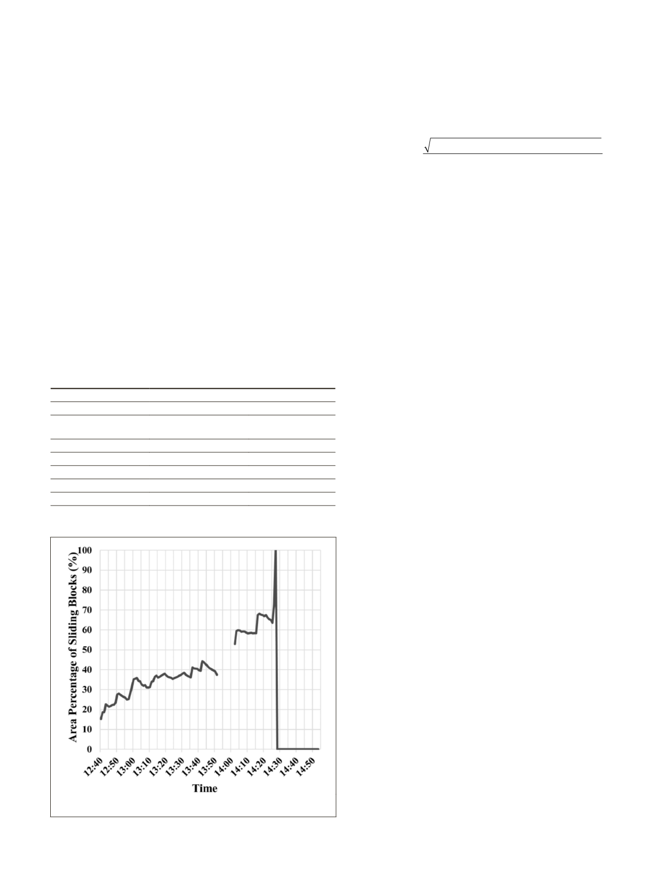
the simulation experiment. Figure 2 presents the percentage
change of the area of sliding blocks during the experiment. A
data gap occurred between 13:52 and 14:03 due to an un-
expected technical problem associated with the simulation
T
able
1. S
pecifications
of
the
C
amera
S
ystems
and
E
xperimental
S
ettings
Items
SLRC
HSCS
Sensor
CCD
CMOS
Image size
2896×1944 pix
1
23.6×15.8 mm
2352×1728 pix
17.4×12.8 mm
Native image bands
RGB
Monochromatic
Focal length
35 mm
20 mm
Starting time
12:40
14:27:22.00
Ending time
14:53
14:27:26.75
Collection frequency
6 frames/min
20 frames/s
1
The maximum resolution of this camera was not used due to the size
limitation of the memory card.
Figure 2. Percentage of the area of sliding blocks versus imaging
time as derived from the sequence of SLRC images.
PHOTOGRAMMETRIC ENGINEERING & REMOTE SENSING
July 2016
551


