HSCS
images in Plate 3 are generally smaller than those from
the
SLRC
image sequence (Figure 3). This finding is mainly
attributed to the fact that the displacement captured by two
adjacent
HSCS
images is generally smaller than that captured
by two adjacent
SLRC
images because of the higher imaging
rate (or shorter time interval, 0.05 sec versus 10 s). Conse-
quently, fewer changed features were detected, and the
P
CF
values were lower. Plate 3 provides a microscopic view of
the short five-second slope failure process. This slope failure
process is merely a spike in Figure 3, but the high-speed imag-
ing and dynamic image processing allow us to visualize it as
a three-stage process. The
P
CF
of the overall slope (grey line)
first sharply increased from 2.4 percent to approximately 28
percent within approximately 1.5 sec, indicating a fast expan-
sion of the deformation area. This expansion was followed by
a short, high-level period of approximately 0.75 sec during
which the
P
CF
value was approximately 26 percent; this period
presents the maximum extent of the movement during the
slope failure. The
P
CF
then gradually decreased from ~26 per-
cent to ~10 percent over the final stabilization stage of 2.5 s.
The
P
CF
patterns of the three sections in Plate 3 can be used
to analyze the dynamics of slope failure. In the first stage,
the most active portion of the landslide body was the middle
section (Section 2); the
P
CF
value of this section was initially
approximately 2.4 percent and increased to approximately
9.3 percent within a half second, followed by brief stabiliza-
tion (yellow curve in Plate 3). This initial deformation of the
middle section led to a larger-scale local collapse of the lower
section (Section 1), as indicated by the very rapid and slightly
delayed
P
CF
increase to 12.5 percent in Section 1 (blue curve in
Plate 3). As a result of the interaction, this local collapse in the
lower section triggered an accelerated collapse in the middle
section, which exhibited an increase in
P
CF
to approximately
13.9 percent (yellow curve in Plate 3). By that time, the gradual
deformation in the upper portion (Section 3) reached a maxi-
mum
P
CF
of 3.5 percent (red curve in Plate 3), after which the
P
CF
of all sections decreased until the end of the experiment.
Surface Velocity Fields during the Final Failure Process
3D instantaneous surface velocity fields are important for
understanding the causes of the final failure process. In the
simulated landslide experiment, the above velocity estima-
tion procedure was performed for all stereo pairs of the
HSCS
stereo-image sequence. Furthermore, an instantaneous
average speed of all sliding features derived at times
t
k
was
calculated. These average speeds (
v
avg
) during the entire slope
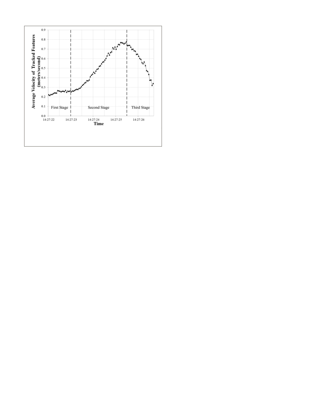
failure process are plotted in Figure 4. The
v
avg
value ranges
from 0.2 m/s to 0.8 m/s, which is reasonable considering the 6
m length of the slope and the slope failure period of less than
five seconds. The speed of most landslides in western China
falls within this range after adjustment for the differences
between the model and actual landslides.
We separated the speed curve in Figure 4 into three stages.
In the first stage (14:27:22.00 to 14:27:23.00), the
v
avg
value was
relatively stable between 0.2 m/s and 0.3 m/s. Then, the speed
accelerated to nearly 0.8 m/s in the second stage (14:27:23.00
to 14:27:25.50). Finally, the speed slowed to 0.3 m/s in the
final stage (14:27:25.50 to 14:27:26.75). The speed trend in
Figure 4 appears similar to the trend of the changed features
in Plate 3; however, a lag of 1.5 seconds occurred from the
peak of
P
CF
value to the
v
avg
maximum. This suggests that the
largest portion of the landslide body moved and then continu-
ously moved to accumulate energy (Plate 3) until the
v
avg
value
accelerated and reached its maximum (Figure 4). In the last
stage, both the
P
CF
and
v
avg
values decreased, suggesting re-
stabilization of the landslide body following its energy release.
To analyze the spatial distribution of the velocity changes
in the entire landslide body during the failure process, speed
maps were generated with a time interval of 0.05 seconds. In
each map, the velocity vectors derived from the sliding features
were first interpolated into a velocity field using the natural-
neighbor interpolation method (Cai and Zhu, 2004) and were
then overlaid onto the landslide body in a GIS system. Note
that the sliding features were pre-filtered to remove abnormal
points before the interpolation was applied. Plate 4 shows the
speed maps with a selected time interval of 0.5 seconds.
In Plate 4, the velocity field was initially limited only to
a small region just above the fissures in the middle section
of the landslide body (time: 14:27:22.00). Then, the veloc-
ity field expanded to the lower-right side (time: 14:27:22.50)
and reached the toe of the slope in the lower section (times:
14:27:23.00 and 14:27:23.50). The speed up until this point
was generally less than 0.4 m/s. Subsequent expansion of
the moving area to the top of the upper section was observed
at time 14:27:24.50. The highest speed occurred near time
14:27:25.50, consistent with the time of the maximum
v
avg
value in Figure 4. The slope body subsequently transitioned
to a balanced state. The moving area decreased and mainly
concentrated in the middle section. In the failure process
represented by the speed maps in Plate 4, “hot spots” with
high speeds that represent local collapses of the slope are ap-
parent. Overall, the temporal changes in the speed maps are
consistent with the
v
avg
curve in Figure 4.
Accuracy
Thirteen well-distributed marked points (Plate 2f) fixed on
the frame of the slope body were established as GCPs. Their
coordinates were measured by a Sokkia total station with an
accuracy of ±1 mm. Eight of these GCPs were then used to
estimate the interior orientation parameters (principal point,
focal length, and lens distortion parameters) and exterior
orientation parameters using the PhotoModeler system
(PhotoModeler, 2013). The estimated accuracy of the exterior
orientation parameters given by the PhotoModeler system
includes: (a) 0.3 mm in the X (horizontal) and Z (vertical)
directions, and 0.4 mm in the Y (depth) direction for the
camera center; and (b) 0.006 degrees, 0.021 degrees, and
0.018 degrees for the orientation angles about the X, Z and Y
coordinate axes, respectively. Furthermore, these eight GCPs
were re-measured in four stereo-image pairs that are evenly
spaced in the sequence of 95
HSCS
image pairs (the 1
st
, 30
th
,
60
th
, and 90
th
stereo-image pairs); their ground coordinates
were photogrammetrically triangulated and compared with
the GCP coordinates; the calculated RMSEs of the ground
Figure 4. Average instantaneous speed (
v
avg
) of the sliding fea-
tures derived from the stereo HSCS image sequences during the
slope failure process.
PHOTOGRAMMETRIC ENGINEERING & REMOTE SENSING
July 2016
553


