PE&RS August 2014 - page 769

dation subsets. This would be computationally intensive, but
yield the most robust two-band HVI.
The Principal Component Regression approach is the poor-
est of the three methods and includes explanatory informa-
tion from the largest number of HNBs in each component. Its
lower performance in the validation dataset reflects the diffi-
culty in choosing components in the final score. The strength
of this method may therefore not be in prediction, but in data
reduction. Future studies could use PCA as a filter to identi-
fy potentially important bands, before implementing SSMs,
which initially have restrictions on the number of predictors.
But, there would still be the issue in selecting the number of
components to include and an additional issue of deciding a
loading threshold in which to include HNBs.
Previous ground-based studies confirm many of the results
of this study, as well highlight the potential of the approach-
es developed in this paper for space-borne hyperspectral
missions. Nguyen and Lee (2006) use PCR analysis to show
that rice growth is highly correlated to pigment absorption
in the visible (524 to 534 nm) and red-edge (687 nm), and
scatter in the NIR (760 to 1100 nm). Our study reveals in each
model-building approach, however that NIR/SWIR bands just
beyond 1100 nm (spectral limit of the previous study) are also
highly significant. Bai et al. (2007) confirms similar correla-
tions between hyperspectral regions and cotton biomass, with
high negative correlations in the visible and relatively lower
negative correlations around the green-peak (510 nm), high
positive correlations in the NIR, and negative correlations in
the SWIR. In particular, models show high correlations with
biomass in the red-edge (672 nm) and NIR (901 nm). Unlike
this study, important SWIR1 (1466 nm) and SWIR2 (2096 nm)
bands are identified as well. Short-wave channels are not
included for cotton in this study, either because the SWIR
channels tended to be more noisy or due to methodological
differences of the two studies. The previous study selected
single bands with the highest biomass variation coefficient
correlation in each spectral region and then built single band
or two-band HVI models around these bands, whereas in
this study, several approaches are evaluated and bands are
selected iteratively with minimal bias. Gnyp et al. (2014) took
a similar methodological approach as this study for rice. Like
this study, the first derivative transformed two-band HVI in-
cluded visible green (526 nm), but explained a lower amount
of variability on their validation subset (R2 = 0.58). Unlike this
study, their best SSM model included six bands in the visible
green, red, and NIR, yet only accounted for 72 percent of the
variability in rice biomass. While our SSM model explained
the same amount of variability using only one variable in the
longer portion of the NIR. Thenkabail et al. (2000) used an SSM
approach to show that the best biomass band for maize is at
the red-edge (654 nm), followed by visible bands (410 and
496 nm), and finally NIR (954 nm), yielding an R 2 of 0.78 with
four predictors. The relatively strong (poor) performance of
maize biomass in the SWIR (red-edge/NIR) in this study, points
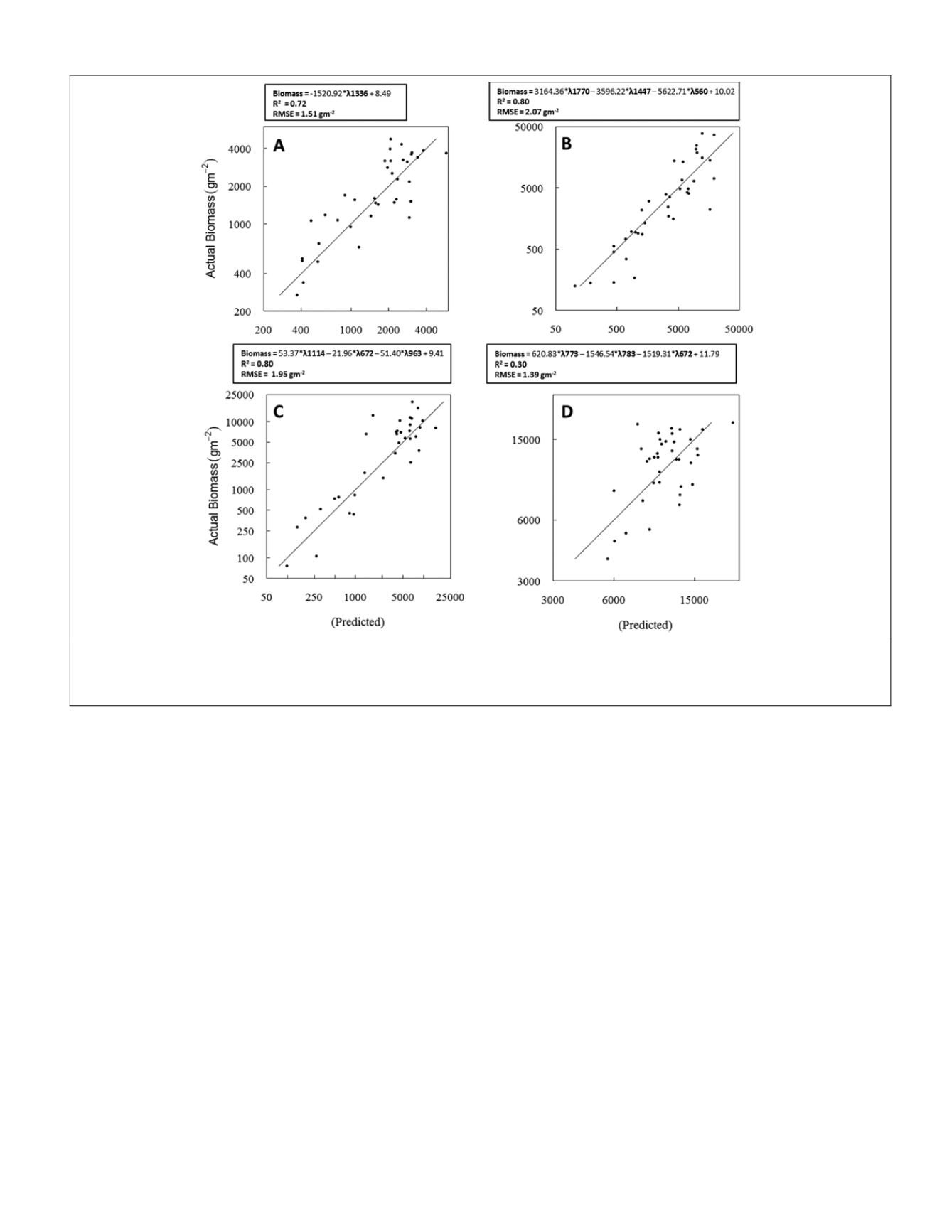
Figure 5. Scatterplots of observed biomass versus predicted biomass for ssm model using the validation subset for (A) rice, (B) alfalfa,
(C) cotton, (D) and maize. The diagonal line represents a 1:1 relationship. Band centers in each prediction equation are preceded by
λ. With the exception of cotton, which is untransformed, equations are built on first derivative transformed spectra.
PHOTOGRAMMETRIC ENGINEERING & REMOTE SENSING August 2014 769