When c
S
falls outside S (like in U-shaped objects), the
proposal of Möller
et al.
(2013) uses an alternative normaliza-
tion factor such as the square root of the area of A
S
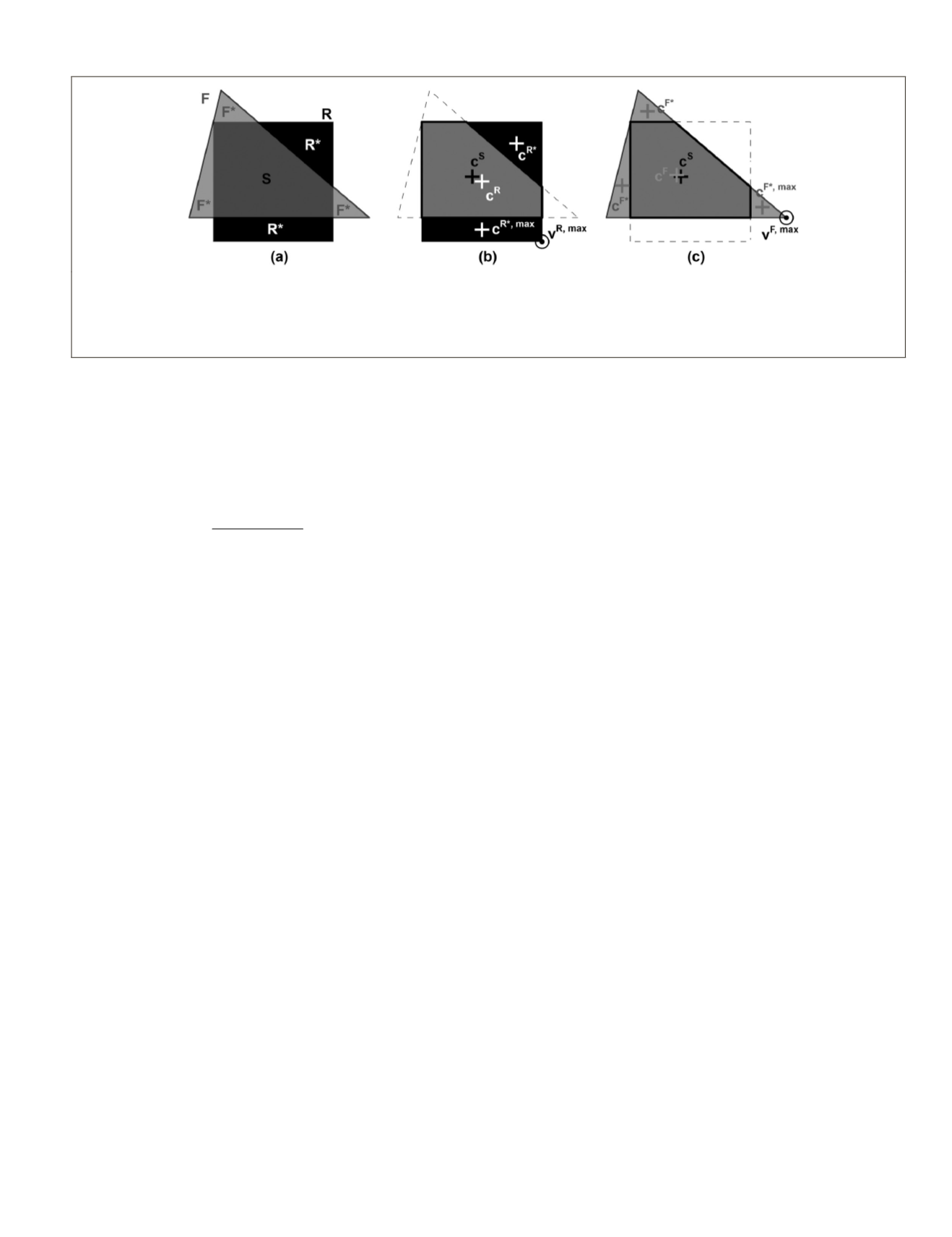
. To avoid
inconsistent formulas that depend on the objects’ shape, in
this paper another normalization factor was implemented
regardless of the object’s shape, which is the distance between
c
R
or c
F
and their respective furthermost vertex of R (v
R,max
) or F
(v
F,max
) (Figure 2b, and 2c). Thus P
R
and P
F
were calculated as:
P
dist c c
dist c v
X
S X
X X max
= −
1
( , )
( ,
)
,
with X
∈
[R,F]
(2)
Next, metrics O
X
and P
X
, with X
∈
[R, F], are combined
through geometric averaging, defining the metrics G
R
and G
F
as G
X
=
√
O
X
P
X
, with X
∈
[R,F]. Metrics G
R
and G
F
assess areal
and positional geometric accuracy of object S in relation to
R and F. Over-segmented and under-segmented objects will
correspond to low values of G
R
and G
F
, respectively. The value
derived for these lie on a scale between 0 and 1.
Finally, all of the G
R
and G
F
metrics are used to calculate
the global metric M
g
for the whole segmentation to measure
the strength and type of mismatch (i.e., under- or over-seg-
mentation) between the reference dataset and the segmenta-
tion. For this, normalized distances D between the cumulative
distribution functions of G
R
and G
F
are calculated by applying
the non-parametric Kolmogorov-Smirnov (
KS
) goodness-of-fit
test, which may be used to assess the difference between two
distributions. Thus, D
+
=max
+
|f(G
F
)-f(G
R
)| and D
–
= max
-
|f(G
F
)-
f(G
R
)|. M
g
results from the difference between D
–
and D
+
. M
g
<0
indicates under-segmentation while M
g
> 0 represents the op-
posite case of over-segmentation. Therefore, M
g
~0 is considered
indicative of optimal segmentation quality (Möller
et al.,
2013).
Furthermore, Möller
et al.
’s (2013) method undertakes a
filtering operation to define the set of objects S considered in
the analysis. Spatial intersection operations commonly cre-
ate narrow and long shapes known as sliver polygons (Mas,
2005). Sliver polygons are often not relevant to the analysis,
as they may appear not from a relevant difference between
the segmentation and the reference but due to minor errors of
geolocation of either one or both layers. For this reason they
are undesired. In the original approach proposed by Möller
et al.
(2013) sliver objects S are referred to as emerging from
many-to-many relations between R and F and are discharged
from all calculations, which happens also in this paper. All
other (non-sliver) objects S are included in the analysis. More
details are found in Möller
et al.
(2013).
Thematic Similarity Index (
TSI
)
The
TSI
was designed specifically in the framework of the
present research to assess the thematic quality of the objects
generated from a segmentation analysis according to the per-
spective of the specific user. The thematic quality of an object
depends on three features: (a) the thematic classes the object
encompasses when its borders are projected on the Earth’s
surface, as represented by the reference dataset, (b) the pro-
portion of the area occupied by each of the classes within the
object, and (c) the thematic similarity between those classes,
which is user dependent. The
TSI
is calculated for each object
of a segmentation as follows:
TSI
P P w
c
n
c
d
n
d cd
=
= =
∑ ∑
1
1
(3)
where
n
is the number of thematic classes within the object,
P
is the relative area (proportion) occupied by each class, and
w
is
the user-specific thematic similarity weight between the classes.
The
n
classes encompassed in the object and the proportion
of area
P
they occupy are defined by a basic spatial overlay
operation between the segmentation under evaluation and the
reference dataset. Thematic similarity is a more complex fea-
ture since the weights
w
are provided by the user and should
express their views on the relative similarity of classes. For
example, if an object is under-segmented and instead of being
pure contains two or more classes, the value of
w
reflects the
relative severity of this error for the specific user.
The description and quantification of thematic similarity
between classes is an issue that has received considerable
attention in the literature. For example, Ahlqvist and Gahegan
(2005) describe methods to estimate the semantic similarity
between any two classes by means of quantitative metrics.
Specifically, they describe how the definition of classes and
their (dis)similarity may be represented by a rough-fuzzy set
approach applied to the defining characteristics that practitio-
ners use to describe or define the classes, such as percentage
of tree cover for a forest. The quantitative metrics used by the
authors are “overlap” and “nearness” which are based on two
common approaches to estimate similarity between concepts:
the proportion of shared features (Tversky 1977) and the psy-
chological distance between related properties (e.g., Nosofsky,
1986). Many other metrics are available in the literature, such
as those described in Bouchon-Meunier
et al.
(1996). More re-
cently, discussion has been introduced in the
GEOBIA
commu-
nity on ontologies (Arvor
et al.
, 2013), which can be useful to
assist the measurement of thematic similarity between classes.
The specific approach adopted can depend of the application
in-hand. Critically, the
TSI
simply requires a pair-wise com-
parison between all land cover classes of interest that yields
a quantitative expression of their thematic similarity. The
derived values can then be summarized in a matrix (Figure
3) and used as weights
w
. The weights that form the matrix
Figure 2. Spatial operation and features considered in Möller
et al.
(2013) for the calculation of geometric metrics: (a) spatial intersec-
tion S between R and F, (b) comparison between S and R, and (c) comparison between S and F. R is a reference polygon; F is an object
of a segmentation under evaluation; S=R∩F; R*=R∩
¬
F; F*=
¬
R∩F; c
R
, c
F
, and c
S
are the centroids of R, F, and S respectively; c
R*,max
is the
furthermost centroid of R* from c
S
; c
F*,max
is the furthermost centroid of F* from c
S
; v
R,max
(alternative to c
R*,max
) is the furthermost vertex of
R from c
R
, and v
F,max
(alternative to c
F*,max
) is the furthermost vertex of F from c
F
.
PHOTOGRAMMETRIC ENGINEERING & REMOTE SENSING
June 2015
453


