PE&RS November 2015 - page 875

Methods
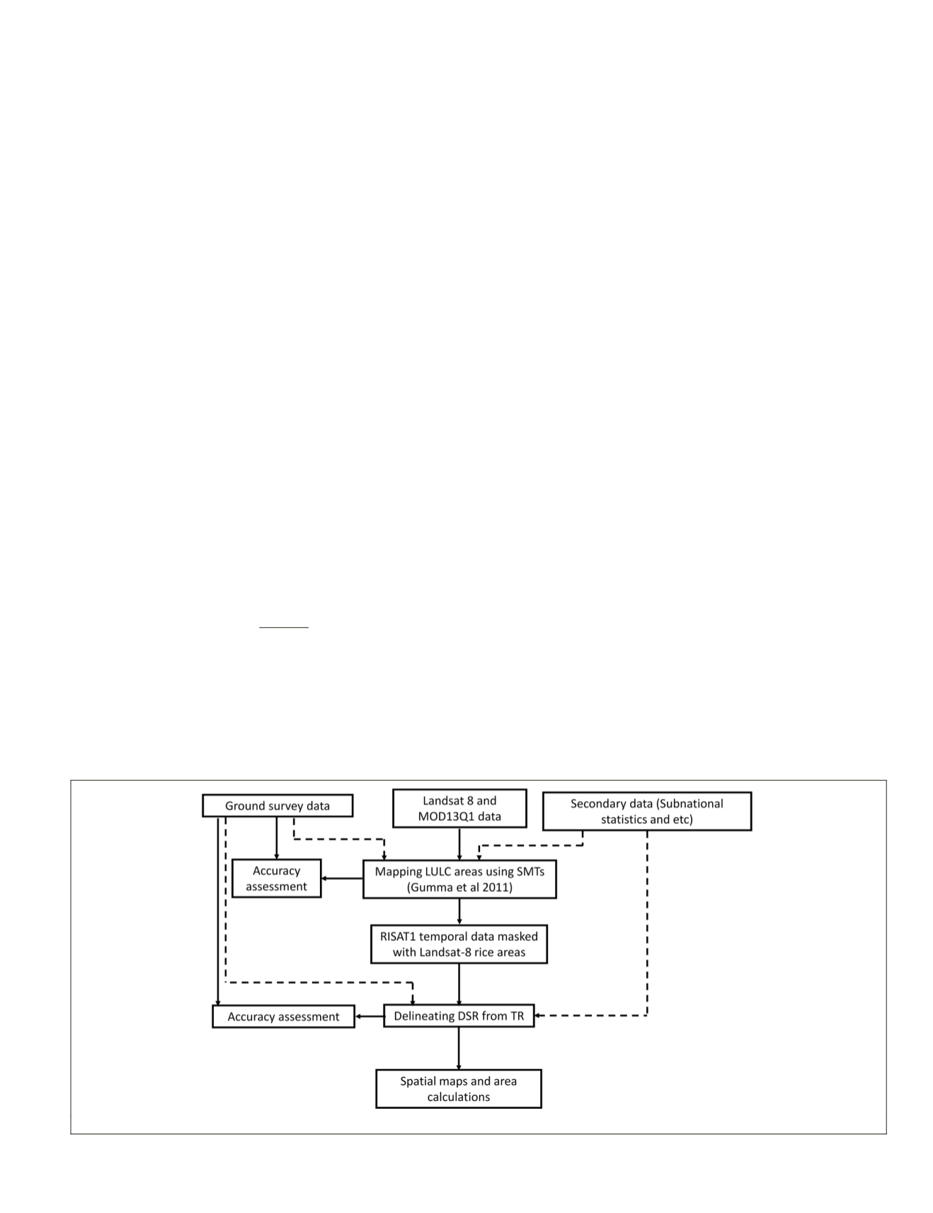
Figure 2 presents an overview of the comprehensive meth-
odology used to map direct seeded and transplanted rice
cultivation practices using time series imagery from MOD09Q1
(spatial resolution 250 m) 16-day time-series NDVI , Landsat-8
(spatial resolution 30 m), and RISAT-1 (spatial resolution 18 m).
Rice growing areas were delineated initially with MODIS time-
series NDVI using spectral matching techniques (Gumma et
al., 2011b; Gumma et al., 2014; Thenkabail et al., 2007a). This
was used as a mask to clip Landsat-8 time-series imagery. The
subset of Landsat-8 was reclassified to separate rice from non-
rice areas due to the difference in resolution between MODIS
and Landsat-8. The Landsat-8 output provided a more ac-
curate delineation of rice growing area. This subset was again
used as a mask to clip out RISAT-1 temporal imagery.
Land-Use / Land-Cover Classification
The procedure began with image normalization of Landsat-8
data converted to top of atmosphere (TOA) reflectance using a
reflectance model implemented in ERDAS Imagine(http://land-
sat.usgs.gov/documents/Landsat8DataUsersHandbook.pdf).
The (Operational Land Imager) OLI band data can be con-
verted to TOA planetary reflectance using Reflectance rescaling
coefficients provided in the product metadata file. The follow-
ing equation was used to convert DN values to TOA planetary
reflectance for OLI data:
ρλ′ = Mρ Qcal + Aρ (1)
where: ρλ′ = TOA planetary reflectance (without correction of
solar angle), Mρ = Band specific multiplicative rescaling factor
from the metadata, Aρ = Band specific additive rescaling factor
from the metadata, and Qcal = the quantized and calibrated
standard product pixel values (DN).
TOA reflectance with correction for the sun angle is then:
ρλ = ρλ
θ
'
sin( )SE
(2)
where: ρλ = TOA planetary reflectance, ρλ′ = TOA planetary
reflectance (without correction of solar angle), and θ SE = the
local sun elevation angle provided in the metadata.
The MODIS stacked composite was classified using unsuper-
vised ISOCLASS cluster K-means classification algorithm fol-
lowed by successive generalization (Biggs et al., 2006; Gumma
et al., 2011c; Thenkabail et al., 2005). The unsupervised
classification algorithm (in ERDAS Imagine 2010) was applied
on a 12-band NDVI (monthly Maximum Value Composite)
MVC to obtain the initial 100 classes, followed by progressive
generalization (Cihlar et al., 1998). The unsupervised classifi-
cation was set at a maximum of 100 iterations with a conver-
gence threshold of 0.99 (Leica, 2010). Time-series NDVI spectra
were then plotted for each of the 100 classes and compared
with the ideal spectra to identify and label classes (Gumma et
al., 2014). However, the time-series NDVI profile helps gain an
understanding of the growth profile of different crops in addi-
tion to providing information on planting date, discrimination
between rice and other crops, early stage conditions (flooded
pixel showing low values initially), and discrimination be-
tween irrigation sources (e.g., irrigated versus rainfed). Class
identification and labeling were performed based on a suite of
methods and ancillary data, such as decision tree algorithms,
spectral matching techniques, Google Earth™ high-resolution
imagery and ground survey data (Gumma et al., 2014; Thenka-
bail et al., 2009b; Thenkabail et al., 2007b). The initial reduc-
tion in classes used a decision tree method (De Fries et al.,
1998) based on the temporal NDVI data. The decision tree is
based on NDVI thresholds at different stages in the season that
define vegetation growth cycle, and these algorithms help to
identify similar classes. The dates and threshold values were
derived from the ideal temporal profile (Gumma et al., 2014).
Using the ground survey data, Google Earth’s high-resolution
imagery along with spectral profiles of rice crops from MODIS
imagery, Landsat-8 imagery was classified using the super-
vised maximum likelihood classification algorithm.
The MODIS -derived rice area was used as the basis of the
maximum possible extent of rice area as one segment and
other LULC areas as another segment. This was used as a mask
to clip Landsat-8 time-series imagery. The subset of Landsat-8
was classified again to separate rice from non-rice areas. Both
segments were classified independently (to avoid mixed clas-
sification) using the protocols mentioned earlier. This led to
a more accurate delineation of rice growing area, but did not
show fragmented direct seeded rice areas. This was mainly
because direct seeded rice was sown in the early monsoon,
when there were no images due to heavy clouds. Landsat-8
rice area was again used as a mask to clip out RISAT-1 temporal
imagery. Separating the two practices of rice cultivation was
possible using RISAT-1 temporal imagery. This is the best com-
plimentary data to monitor croplands during the monsoon
season, and where there are continuous clouds.
Figure 2. Overview of the methodology for mapping different rice growing practices.
PHOTOGRAMMETRIC ENGINEERING & REMOTE SENSING November 2015 875