where
R
2
is the determination coefficient indicating the accu-
racy of the method, with = 0.02 and = 0.651. The two-band ratio
method makes it easier to retrieve water vapor content from sat-
ellite images without any
in situ
data or simulated coefficients.
Simulation of the Relationship between Water Vapor and Atmospheric
Transmittance
It is difficult to directly estimate atmospheric transmittance
from satellite data or other atmospheric data. In general, atmo-
spheric transmittance is acquired through simulation using
local atmospheric data, especially water vapor content. Simu-
lation of the relationship between atmospheric transmittance
and water vapor can be built through atmospheric modeling
programs such as
MOD
erate resolution atmospheric
TR
ANs-
mission (
MODTRAN
).
MODTRAN
(Berk
et al.
, 2006) is a “narrow
band model” atmospheric radiative transfer program, and its
spectral range extends from the ultraviolet into the far-infrared
(0 ~50000 cm
-1
), with a spectral resolution of up to 0.2 cm
-1
.
In the Antarctic, the volume of water vapor is much lower
than other regions, and it contributes little to the annual pre-
cipitation. According to the observation data, the minimum
and maximum values of water vapor were set as 0.05 g/cm
2
and
3.0 g/cm
2
, respectively. For this range of water vapor content,
the relationship between water vapor content and atmospheric
content is approximately nonlinear. Thus, a series of polyno-
mial fitting functions were used to describe the relationship be-
tween transmittance and water vapor, replacing the traditional
linear fitting. Please see the next Section for more details.
Results and Discussion
Algorithm Validation
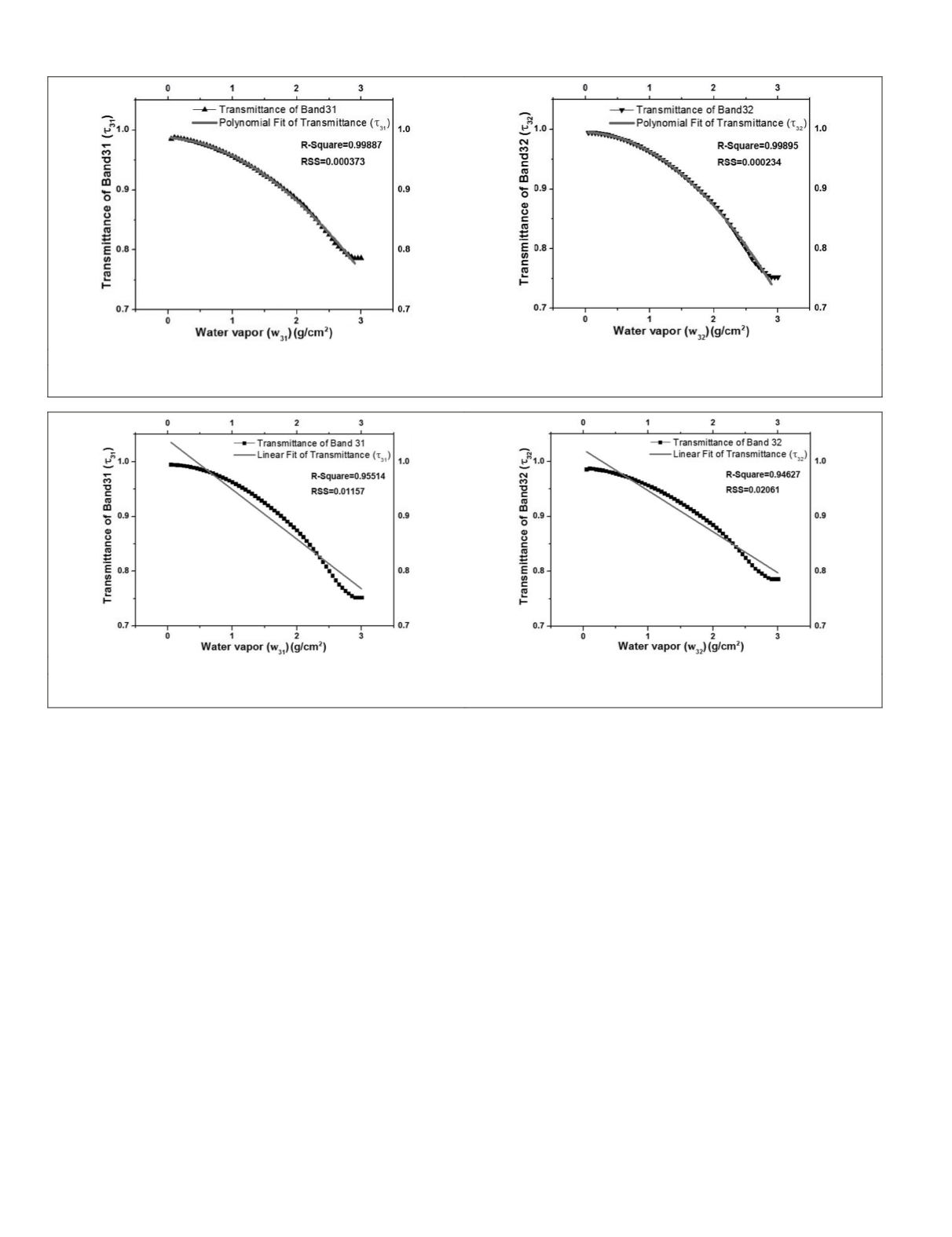
The fitting results of the relationship between water vapor con-
tent and atmospheric transmittance are presented in Figure 4
.
In Figure 4a and 4b, the dotted lines show the change
trend of the atmospheric transmittance with the increase in
water vapor in the two
MODIS
thermal channels, bands 31 and
32, respectively. As the water vapor increases, the atmospher-
ic transmittance decreases sharply. Within this range, water
vapor has presented a linear relationship with atmospheric
transmittance in most of the previous studies (Qin
et al.
,
2001; Mao
et al.
, 2005). However, in this study, it was found
that this relationship can be better represented by a polyno-
mial function. The solid lines in Figure 4 a and 4b show the
results of polynomial fitting, and the corresponding polyno-
mial equations are provided as follows:
τ
31
= 0.9955 – 0.00299 ×
w
31
– 0.02926 ×
w
31
2
(9)
τ
32
= 0.98822 – 0.00902 ×
w
32
– 0.02193 ×
w
32
2
(9)
In Figure 4, higher determination coefficients (R
2
) corre-
spond to more accurate results. A small value for the residual
sum of squares (
RSS
) also indicates a relatively high accuracy.
The accuracy for the linear-fitting-based regression analysis
and the fitting results are provided in Figure 5.
The lower accuracy and the linear fitting results in Figure
5 indicate that the linear fitting cannot accurately describe the
(a)
(b)
Figure 4. The polynomial fit of the relationship between water vapor content (
ω
) (g/cm
2
) and atmospheric transmittance (
τ
ω
): (a) Band 31
polynomial fitting result, and (b) Band 32 polynomial fitting result.
(a)
(b)
Figure 5. The linear fit of the relationship between water vapor content (
ω
) (g/cm
2
) and atmospheric transmittance (
τ
ω
): (a) Band 31 linear
fitting result, and (b) Band 32 linear fitting result.
866
November 2015
PHOTOGRAMMETRIC ENGINEERING & REMOTE SENSING


