Niclòs
et al.
, 2007; Vincent, 2000) and
LST
retrieval (Price,
1984; Tang
et al.
, 2008; Xiao
et al.
, 2008; Peña, 2009; Nichol,
2009; Rajasekar and Weng, 2009; Jimenez-Munoz
et al.
, 2014)
.
The
SWA
used in the
MOD
29 retrieval procedure is imple-
mented as a regression model, which can be described as the
following equation (Hall
et al.
, 2004):
T
S
=
a
+
bT
31
+
c
(
T
31
–
T
32
) +
d
[(
T
31
–
T
32
)(sec
θ
– 1)] (1)
where
T
s
is the surface temperature;
T
31
and
T
32
are the bright-
ness temperatures of bands 31 and 32 in the
MOD
021KM data,
respectively;
θ
is the sensor scan angle; and
a
,
b
,
c
, and
d
are
the regression coefficients. In this procedure, large quantities
of
in situ
data are used to determine the empirical relation-
ship and its corresponding coefficients in Equation 1 through
a least squares regression method
.
In this research, an improved
SWA
was used to imple-
ment the
MODIS
-based
IST
retrieval in the Antarctic area. This
improved version of
SWA
, which was developed by Qin
et al.
(2001), requires only two essential parameters (emissivity and
transmittance), and can be described as the following simple
regression function:
T
S
=
A
0
+
A
1
T
31
–
A
2
T
32
(2)
where
A
0
,
A
1
, and
A
2
are the coefficients, which are deter-
mined by the atmospheric transmittance, the ground emissiv-
ity, and viewing angle:
A
a D C D
D C D C
a D C D
D C
0
31 32
31
31
32 31
31 32
32 31
32
32
32 3
1
1
=
− −
(
)
−
(
)
−
− −
(
)
1
31 32
−
(
)
D C
(3)
A
D
D C D C
b D C D
D C D C
1
31
32 31
31 32
31 32
31
31
32 31
31 32
1
1
= +
−
(
)
−
− −
(
)
−
(
)
(4)
A
D
D C D C
b D C D
D C D C
2
31
32 31
31 32
32 31
32
32
32 31
31 32
1
=
−
(
)
+
− −
(
)
−
(
)
(5)
where a
31
=−64.60363, b
31
=0.440817, a
32
=−68.72575,
b
32
=0.473453, and
C
i
=
ε
i
τ
i
(
θ
)
(6)
D
i
= [1 –
τ
i
(
θ
)][1 + (1 –
ε
i
)
τ
i
(
θ
)]
(7)
where
τ
i
(
θ
) is the atmospheric transmittance of the
i
th
band (
i
= 31, 32) on the sensor scan angle
θ
, and
ε
i
is the surface emis-
sivity of the
i
th
band (
i
= 31, 32)
.
Equations 6 and 7 indicate that the key steps in this
method refer to emissivity acquisition and transmittance
estimation. This makes it easier to retrieve
IST
without the
complicated estimation of other coefficients and parameters.
Surface Emissivity
Surface emissivity is defined as the ratio of the radiant energy
of an object to the radiant energy of a standard black body at the
same temperature. It reflects the different physical characteris-
tics of different land-cover types. Ice/snow surface emissivity is
a key parameter for
IST
retrieval (Warren, 1982; Key and Hae-
fliger, 1992). Several spectral libraries are available for various
types of terrestrial surface emissivity, such as the
ASTER
(the
Advanced Spaceborne Thermal Emission Reflection Radiom-
eter) Spectral Library (Baldridge
et al.
, 1999) and the
MODIS UCSB
(University of California, Santa Barbara) Emissivity Library (Wan
et al.
, 1994). A number of field campaigns have also been car-
ried out to measure ice/snow emissivity (Hori
et al.
, 2006; Key
and Haefliger, 1992). Emissivity varies with ice/snow surface
conditions, such as surface melt (Hori
et al.
, 2006; Salisbury
et
al.
, 1994; Wald, 1994), snow grain size (Stroeve
et al.
, 1996), and
sensor scan angle (Key and Haefliger, 1992; Hori
et al.
, 2006).
According to Stroeve
et al.
(1996), a 0.1 percent bias in emis-
sivity corresponds to a 0.1 K deviation in
IST
. In this study, the
emissivity over the Antarctic was set to 0.993 (for band 31) and
0.990 (for band 32), referring to the research of Hall
et al.
(2008).
Atmospheric Transmittance
Atmospheric transmittance describes the magnitude of the
thermal radiance (
TR
) attenuation. Attenuation occurs under
the influence of the atmospheric constituents and atmo-
spheric scattering when the
TR
is transferred to sensors. The
atmospheric constituents, such as N
2
, O
3
, and CO
2
, are rela-
tively stable; therefore, their influences can be assumed to be
constant and can be simulated by the standard atmospheric
profiles (Qin
et al.
, 2001). Aerosols can result in atmospheric
scattering, but their influence on
TR
transfer is insignificant
considering their low level in the atmosphere. In contrast, wa-
ter vapor significantly contributes to
TR
attenuation. The vari-
ance of atmospheric transmittance depends on the dynamic of
the water vapor content in the standard atmospheric profiles.
Therefore, atmospheric transmittance can be estimated by
simulating its relationship with water vapor content.
Water Vapor Retrieval
Various approaches (Chesters
et al.
, 1983; Kleespies and Mc-
Millin, 1990; Birkenheuer, 1991) have been proposed for water
vapor retrieval. The satellite-data-based approaches focus on
the absorption of water vapor when the reflected solar radi-
ance is transferred down to the land surface and up through
the atmosphere (Kaufman and Gao, 1992). In Kaufman’s
research (1992), the relationship between transmittance (
τ
w
)
and the total precipitable water vapor (
w
) was defined as the
ratio of several bands. This principle is based on the differ-
ence between the atmospheric absorption and the atmospheric
window. In this study, a two-band ratio approach was applied:
τ
w
=
r
i
/
r
j
(8)
where
r
i
is the reflectance of band 19, which is the absorption
band; and
r
j
is the reflectance of band 2, which is the window
band. The relationship between the transmittance and the
total precipitable water vapor (
w
) can be expressed using an
exponential equation:
w
= ((
α
–
ln
τ
w
)/
β
)
2
,
R
2
= 0.999
(9)
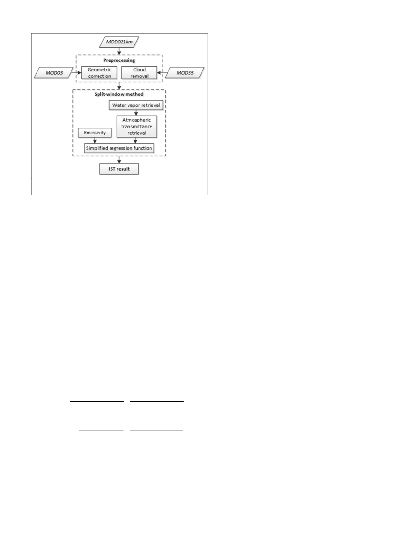
Figure 3. The flowchart of the proposed MODIS-based IST re-
trieval method.
PHOTOGRAMMETRIC ENGINEERING & REMOTE SENSING
November 2015
865


