which result in existence of a high amount of relief displace-
ments towards different directions causing difficulties for
conventional coregistration methods. Also, the images of
datasets DT1 to DT3 are selected from across-sensor imagery
while in DT4 the images are selected from the same satellite.
On the other hand, the sources for the used DSMs are
from either stereo images or lidar as mentioned in Table 2.
The accuracy of the both of DSMs is checked with the avail-
able ground control points and both DSMs have an accuracy
around 0.5m in all directions.
Table 3 shows the spectral band width and the dynamic
range of the satellites whose images are used as across-sensor
datasets (DT1 to DT3).
T
able
3: S
pectral
B
and
W
idth
and
the
D
ynamic
R
ange
of
the
S
atellites
whose
I
mages
are
U
sed
as
A
cross
-S
ensor
D
atasets
in
this
S
tudy
Satellite
NIR
(μm)
Red
(μm)
Green
(μm)
Blue
(μm)
Dynamic
Range
Ikonos
0.757-0.853 0.632-0.698 0.506-0.595 0.445-0.516 11 bits
GEOEYE
0.78-0.92 0.655-0.69 0.51-0.58 0.45-0.51 11 bits
As can be seen, the dynamic ranges for both satellites are
equal to 11 bits and the spectral bands are also very close.
However, slight spectral differences still exist in the across-
sensor bi-temporal combinations, which could affect the
change detection results.
Radiometric Normalization
Before performing any change analysis, it is necessary to es-
tablish a radiometric normalization between bi-temporal im-
ages to attenuate the radiometric differences caused by effects
such as atmospheric conditions and sensor gains. Since the
images used in this study are already corrected for atmospher-
ic effects and the solar illumination angles of the bi-temporal
sets are similar (Table 1), a linear relation between the intensi-
ties of corresponding patches seems reasonable for radiomet-
ric normalization.
Typically, radiometric normalization is performed us-
ing the pseudo-invariant pixels/objects taken as reference
(Sohl, 1999; Im and Jensen, 2005) in a supervised manner.
For unsupervised radiometric normalization, Ye and Chen
(2015) proposed a twofold process. In this study, an object-
based version of their process is used. Here, after the
PWCR
, a
linear regression is initially fitted to the mean (for shift and
scale) and standard deviation values (for only scale) of the
corresponding patches. Then, the linear coefficients are used
to normalize the target object mean values. After that, it is
necessary to remove the effect of changed patches from the
radiometric normalization regression results, since only the
radiometric values of the corresponding unchanged patches
should be used for radiometric normalization. For this
purpose, using a simple change detection method, the Image
Differencing method, the unchanged patches are detected
and removed from the radiometric normalization process.
Next, a similar new linear regression is fitted to the mean and
standard deviation values of the unchanged corresponding
patches in the base and target images. Finally, all the target
mean values are normalized using the latter generated linear
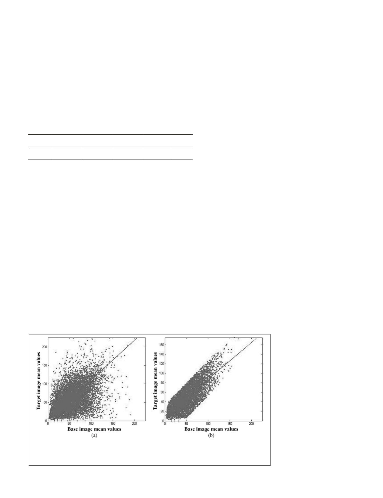
regression coefficients. Figure 7 shows an example of scat-
ter plots of the mean values of the base and target patches
in dataset DT3 (Red band). Figure 7a depicts the initial
mean values and the first regression line. After removing the
changed patches from the radiometric normalization process,
the scatter plot and the final regression line are presented
in Figure 7b. As can be seen, the scatter of the unchanged
patches approximately follows a linear function. Therefore, a
linear regression is suitable for the radiometric normalization
step in our work.
The reason we used both mean and standard deviation in
linear regression is that we estimate the values of the pixels
in each patch by their mean value. However, to have a better
estimate of the scale of linear regression parameters the devia-
tion of the pixels from mean value in each patch can also be
used in this regard.
Results
PWCR Results
Plate 1 depicts examples of the original patches in the base
images, (a), (c), and (e), and the corresponding ones gener-
ated in the target
images, (b), (d), and (f), using the presented
PWCR
method. As can be seen, the borders of the so generated
patches in the target images properly fit the real object bor-
ders. Plate 1b is a part of the target and the older image in the
bi-temporal set DT3. The borders of the buildings, and also
other newly constructed objects which exist in the base image
(Plate 1a), are also transferred to the old image where there
is no construction yet. This process produced empty poly-
gons on the ground in Plate 1b. Plate 1c shows the patches of
a part of the base image in dataset DT1. The corresponding
patches in the target image are
shown in Plate 1d. Plate 1e
shows the roof borders of some
high-elevated buildings in the
base image of dataset DT4. The
corresponding roofs generated
using the
PWCR
in the target im-
age are also shown in Plate 1f.
Plate 2 depicts an example
comparing the results of the
segments transferred from the
base
image to the target
image
,
using the conventional poly-
nomial image-to-image regis-
tration and the
PWCR
method.
Plate 2a presents the manually
generated segments (object
borders) of the base
image in
dataset DT3; in Plate 2b the
same segments are generated in
the target
image using the
PWCR
method; in Plate 2c, 2d), and 2e
the target
image (from dataset
Figure 7. Scatter plot of the mean values of the corresponding patches in the Red spectral band of
Dataset DT3: (a) before, and (b) after removing the changed patches. The regression line in (b) is a
better representation of the relation between the mean values of the corresponding patches in the
base and target images. Therefore, it is used for final radiometric normalization of the patches.
PHOTOGRAMMETRIC ENGINEERING & REMOTE SENSING
July 2016
527


