Morphological Scale Space Filtering
In this study the morphological scale space filtering has been
employed in order to tackle the high spectral variability
and complexity of urban areas. Morphological levelings are
widely considered as a beneficial tool for image scale space
simplification and segmentation (Meyer 2004;Tzotsos
et al
.,
2011). In morphological leveling, the multispectral data are
simplified, without smoothing the object edges that remain
sharp. Image regions with homogeneous spectral behavior,
without important variation, become smoother while the im-
age contours are preserved. Under such a filtering procedure
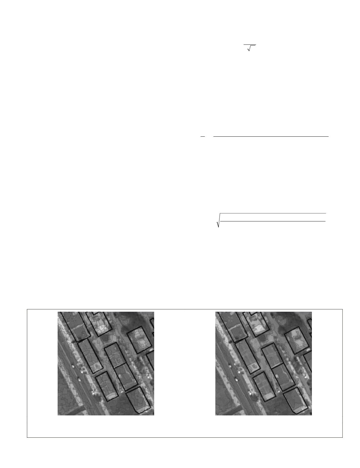
(Figure 2), building boundaries remain clear and detectable in
subsequent segmentation or classification process (Karantza-
los
et al
., 2007; Doxani
et al
., 2012).
Image Segmentation
The first step in object-based image analysis is the image
segmentation process, in order to generate meaningful image
objects. In this study, the multi-resolution segmentation was
performed with Definiens Professional software, through a
bottom-up procedure that starts by treating each pixel as an
object and then merges the neighboring image objects based
on spectral and shape homogeneity criteria (Benz
et al
., 2004;
Definiens, 2010). The segmentation output in this case de-
pends on the parameters of scale, shape, and compactness, de-
fining the object size, compactness, and smoothness, respec-
tively. Since those parameters are user-dependent, they must
be defined by a trial and error process in every case study. The
optimal segmentation parameters are defined in our approach
by testing different combinations and evaluating the segmen-
tation results (Neubert
et al
., 2008; Costa
et al
., 2008; Clinton
et al
., 2010). The employed evaluation criteria are based on
the comparison of the area, the shape and the position of the
ground truth polygons (reference objects) and the correspond-
ing resultant segments inside the reference object:
1. Average difference of the area [percent] (Neubert
et al
.,
2008): The percentage of the area difference between
the reference object and the resulting segments, aver-
aged over all the reference objects.
2. Average difference of perimeter [percent] (Neubert
et
al
., 2008): The percentage of the perimeter difference
between the reference object and the resulting seg-
ments, averaged over all the reference objects.
3. Average difference of shape index [percent] (Neubert
et
al
., 2008): The shape index difference of the reference
object and the resulting segments, averaged over all the
reference objects. The shape index is defined as:
Shape Index
=
P
A
4
(1)
where
P
is the perimeter and
A
, area of the object.
4. Average number of partial segments [percent] (Neubert
et
al
., 2008): The number of the partial segments inside the
reference object, averaged over all the reference objects.
The value indicates the grade of over-segmentation.
5. Fitness Function (Costa
et al
., 2008): The sum of the
area of the pixels that have been “lost” (belong to the
reference but not to the segments) and the ones that
have been “added” (belong to the segments but not to
the reference) averaged over all the reference objects.
For
n
reference objects it is defined as:
F
n
Area of lost pixels Areaof added pixels
Area
i
n
=
+
=
∑
1
1
"
"
"
"
of the referenceobject
. (2)
6. Area Fit Index (Lucieer and Stein, 2002): The proportion
of the area difference between the reference object and
the largest segment over the area of the reference object.
7. Location Quality [
qLOC
] (Zhan
et al
., 2005): The Eu-
clidean distance between the centroids of the reference
objects and the resulted segments.
8. Index D (Clinton
et al
., 2010): It can be considered as a
measure of the closeness to an ideal segmentation and
it is defined as:
Index D
OverSegmentation UnderSegmentation
=
+
2
2
2
. (3)
The selection of the parameters at this stage is important
not only for the optimal segmentation output, but also
for the comparison of different segmentation approaches.
Indeed, in this study the criteria are suitable to compare
the segmentation output of the original and the scale space
images when the same parameters are selected (Clinton
et
al
., 2010). The tested scale parameters are in the range of [10,
50] in steps of 10, and the shape as well as the compactness
parameters are in the range of [0.1, 1], in steps of 0.1. In Table
1 we present the results of the criteria evaluation for the
optimal scale parameters combination (Scale: 20, Shape: 0.3,
(a)
(b)
Figure 2. The reference data (polygons in bold) superimposed on the segmentation results of (a) the original image, and (b) the filtered
image after the scale-space simplification.
PHOTOGRAMMETRIC ENGINEERING & REMOTE SENSING
June 2015
483


