Penalization of false positive image line has been treated as
the modeling of the angular residual error (i.e., angular differ-
ence) between a back-projected wireframe
LM
i
line and all the
candidate image lines
LI
′
. In
SP
,
LI
′
comprises
N
image lines
{
LI
k
}
N
k
=1
where
LI
k
can be found if any member pixel of
LI
k
shows
less than two pixel deviation from
LM
i
. The modeling of the
a priori
error distribution uses a Laplacian probability den-
sity function. The York Urban Database (Denis
et al.
, 2008), a
database of terrestrially captured images comprising of indoor
and outdoor man-made scenes, has been used to perform the
training for parameter definition in the fitting of the distribu-
tion model. From the 102 images in the database, 12 randomly
selected images with reference data lines obtained from man-
ual digitizing were used for training (i.e.,
≈
10 percent of the
dataset). From the 12 images, line segments are then automati-
cally detected. The angular difference between the reference
data lines and the automatically established lines are then
collected. Two lines, i.e., a reference data “model” line and an
automatically detected line are considered to be the same line
if they are less than 1.5 pixels apart in the 640 × 480 images.
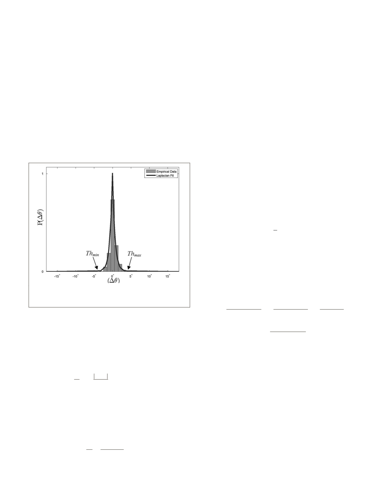
Figure 8. Error model for orientation residual scoring of true
positive line presence, where
Th
min
and
Th
max
are the threshold
bounds of the error function.
Figure 8 shows the function where its ordinate axis is a
normalized scale between 0 and 1. The function, i.e., the
angular residual score
P
ik
(
Δ
θ
),
is defined in Equation 4 with
parameters
b, µ
and
∆
θ
(i.e.,
angular difference between
LM
i
and
LI
k
∈
LI
′
). To model the wireframe to image line angular
deviations, the estimated fitting parameters for the Laplacian
function, where
b
= 0.66,
µ
= −0.04, are:
0
4
∆
θ
∆
θ
(
)
;
,
,
P LM LI
if
Th
or
Th
ik
i
k
min
max
∆
θ
=
≤
= − °
≥
=
4
1
2
1
°
−
−
≤ ≤
,
,
f
b
exp
b
if Th
Th
f
min
max
∆
θ µ
∆
θ
if
∆
θ
=
0
(4)
The Laplacian-based scoring function assigns a relatively
high score if the angular residual between the image and
wireframe lines are small. Likewise, if the residual is high, a
low score will be attributed. The geometric similarity score
function
SP
for a wireframe line is given by Equation 5.
SP LM LI
N
len LI
len LM
P LM LI
i
k
N
k
i
ik
i
k
,
( )
(
)
;
,
’
(
)
=
(
)
=
∑
1
1
∆
θ
(5)
where
len
is line length and the ratio
len
(
LI
k
)/
len
(
LM
i
) =
min(1,
len
(
LI
k
)/
len
(
LM
i
)).
Any
LI
k
that is short is penalized. The ratio of image line
length to the wireframe line length is used as a weighting cri-
terion. This ensures that true positive matching lines that may
be high-scoring angular-wise, but possibly only two or three
pixels in length, are considered less influential in the overall
scoring. If
len
(
LI
k
) is greater than
len
(
LM
i
), then the weighted
length ratio is given a max value of 1. The line similarity
score is obtained for every image line that intersects each
individual wireframe line. The summations of the individual
scores are then averaged by the number of image line pres-
ence candidates,
N
, to obtain a single presence score for
LM
i
.
Evidence 3 - Virtual Corner Presence
We propose a scoring function, called virtual corner presence
SV of Equation 6, for measuring the quality of correspon-
dences of associate lines forming a corner. The line presence
scores of Equation 5 propagate into the confidence scores that
support the corner presence. A set of wireframe corners,
CM
,
which are deemed to be present on the image are referred to
as “virtual corners”
VC
in the image space. For measuring
the quality of virtual corner presence, first we back-project a
wireframe corner
CM
j
∈
CM
and its two associated wireframe
lines {
LM
i
}
2
i
=1
∈
LM
onto the image based on a camera param-
eter hypothesis. Then,
LI
′
, image lines associated with
LM
i
,
are obtained in a similar way previously described. Finally a
single score of corner presence
SV
is computed by averaging
the total scores of individual line presence of the two hypoth-
esized wireframe lines {
LM
i
}
2
i
=1
forming
CM
j
.
SV
(
CM
j
) =
1
2
1
2
i
=
∑
SP
(
LM
i
,
LI
′
)
(6)
Combined Evidence Scoring
The individual scores from the various evidences are com-
bined into a single confidence value to rate the given hypoth-
esis of camera parameters.
E
+
and
E
-
define the positive and
negative evidence scores respectively (Equation 7).
E
-
is the
negative image line pixel coverage. Weights
w
α
,
w
β
, and
w
γ
are
assigned to
E
+
and a bias penalizing weight
w
δ
is applied to
E
-
.
E w
SC LM LI
card LM
w
SP LM LI
card LM
w
CM
car
i
i
j
+
=
(
)
( )
+
(
)
( )
+
∑
∑
∑
,
,
’
’
d CM
(
)
α β γ
(7)
E w
SN LM LI
card LM
j
−
=
(
)
( )
∑
,
'
δ
where,
card ( )
is the cardinality of a set.
The non-matching pixels are only penalized with half
weight value (i.e.,
w
δ
set at 0.5) to account for shadows and
occlusions preventing line extraction and thus being less
biased compared to assigning a full score for
E
-
. The hypoth-
esis score
S
C
is represented by accumulated evidence and is
defined in Equation 8.
S
C
(
E
+
,
E
-
) =
E
+
–
E
-
(8)
The best camera parameter hypothesis
C*
is chosen ac-
cording to the criteria established in Equation 9.
C
* =
argmax S
C
(
E
+
,
E
-
)
(9)
"
{
C
}
The maximum number of
LR-RANSAC
iterations is chosen
as 2000 in all the experiments based on the probability that at
PHOTOGRAMMETRIC ENGINEERING & REMOTE SENSING
November 2015
853


